Examples

GaAs(111) at 800 nm

SHG Simulation

GaAs crystallizes in a cubic structure with the point group $\overline{4}3m$ and its linear and nonlinear optical properties have been extensively studied. In this example, the polarized nonlinear optical response will be simulated and derived both numerically and analytically.

Follow Open the ♯SHAARP.si.nb in the Mathematica® software on your computer to initiate the Mathematica notebook.
Click SHG Simulation in the Functionality section.
Click the dropdown button next to the Case Studies to expand the content in the section.
Click GaAs (111) to update input parameters for Crystal Structure, Crystal Orientation, Linear Optical Tensors and SHG Tensors (d_ijk). The lattice parameters can be found in the CIF file. The complex linear optical properties can be found in RefractiveIndex.Info and the nonlinear optical tensors were evaluated by the Ref. Then click Update to evaluate the new input.
The output results will be shown in the right-hand panel. The Probing Geometry and Polarization Relations shows the orientation of crystals and polarization configuration.

Probing Geometry and polarization settings for GaAs (111)

Here, in the geometry plot, $(L_1,L_2,L_3)$ depicts the lab coordinate system forming a right-handed coordinate, and the normal of surface (111) plane is parallel to the $L_3$ direction. The $L_1-L_3$ forms the plane of incidence (PoI) as colored in blue. The input [hkl]->Direction Perpendicular to Plane of Incidence is set parallel to the $L_2$ direction. In the polarization plot, the both incident polarization at $\omega$ frequency and output SHG polarization at $2\omega$ frequency are rotated simultaneously with a same azimuthal angle $\varphi$ . Two output SHG electric fields (colored in blue and red) with orthogonal polarization are collected.

The intensity of the selected electric fields are plotted as a function of $(\varphi,\Psi)$ and plotted with the same color code as presented in Polarization Relations.

SHG polar plots as a function of $(\varphi,\Psi)$ . The directions of output polarization share the same set of color codes as presented in the Polarization Relations plot.

The Effective refractive index and Ellipticity of incident light at $\omega$ are shown in the third row. In the Effective refractive index plot, the real parts of effective refractive indices are shown as a function of incident angle. Superscript 1 and 2 refer to ordinary and extraordinary waves. In cubic GaAs case, refractive indices are the same regardless of the directions of electric fields. In the Ellipticity plot, the phase relation of $E_p$ and $E_s$ is shown. If linear polarization is rotated, the ellipticity of light will be shown with $\varphi=45^o$ , otherwise the explicit direction of $E^{\omega}$ will be shown.

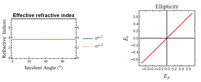Effective refractive index shows the effective refractive indices for both ordinary and extraordinary waves as a function of incident angle at $\omega$ frequency. Ellipticity exhibits phase relations between $E_p$ and $E_s$ at $\omega$ frequency.

SHG Partial Analytical Expressions

Follow Open the ♯SHAARP.si.nb in the Mathematica® software on your computer to initiate the Mathematica notebook.
Click SHG Partial Analytical Expressions in the Functionality section.
Click the dropdown button next to the Case Studies to expand the content in the section.
Click GaAs (111) to update input parameters for Crystal Structure, Crystal Orientation, Linear Optical Tensors and SHG Tensors (d_ijk). The lattice parameters can be found in the CIF file. The complex linear optical properties can be found in RefractiveIndex.Info and the nonlinear optical tensors were evaluated by the Ref. Then click Update to evaluate the new input.
The output results will be shown in the right-hand panel as presented below.
The partial analytical expressions are expressed with SHG coefficients variables and numerical values for the rest of the parameters.
The Copy button next to the equation allow direct copy of the equation to the clipboard.

SHG Full Analytical Expressions

Follow Open the ♯SHAARP.si.nb in the Mathematica® software on your computer to initiate the Mathematica notebook.
Click SHG Full Analytical Expressions in the Functionality section.
Click the dropdown button next to the Case Studies to expand the content in the section.
Click GaAs (111) to update input parameters for Crystal Structure, Crystal Orientation, Linear Optical Tensors and SHG Tensors (d_ijk). The lattice parameters can be found in the CIF file. The complex linear optical properties can be found in RefractiveIndex.Info and the nonlinear optical tensors were evaluated by the Ref. Then click Update to evaluate the new input.
The output result will be shown in the right-hand panel as presented below (this process can take a few minutes, please be patient). You can refer to the progress bar at the top of the panel for current status.

Full Analytical Expressions. Types of variables are color-coded with distinct colors.
The full analytical expressions are expressed with pure variables. The definition of variables can be accessed using the variable table.
The Copy button next to the equation allow direct copy of the equation to the clipboard.

LiNbO₃(110) at 800 nm